Bayesian Factor Modeling for Market Forecasting - Daniel D. McKinnonDaniel D. McKinnon

If you find this post interesting, check out A practical treatise on pairs trading, Bellman-Ford, Shannon’s Demon, and order book pressure: Tales from 18 months of cryptocurrency arbitrage

Introduction

The Capital Asset Pricing Model (CAPM) was introduced nearly 50 years ago to provide a framework with which to analyze the returns of securities (Sharpe 1964). At its core, it decomposed return into a three parameters, a risk-free rate, a market rate, and a coefficient that measures the sensitivity of an individual security’s return to that of the market.

${\mathbb{E}(R)=R_f + \beta(\mathbb{E}(R_m) - R_f)}$ , where ${R_f}$ is the risk-free rate, ${R_m}$ is the market rate, and ${\beta}$ is the sensitivity.

While this model earned its creator, William Sharpe, a Nobel Memorial Prize for Economic Sciences, it did not stand the test of time. Returns of securities could not be decomposed in such a simplistic way. Fifty years later, Eugene Fama and Ken French extended the CAPM model to include additional factors express a security’s sensitivity to company size and book-to-market ratio (Fama 1993). This model served economists and portfolio managers well for almost 20 years before being replaced by an updated 5-factor model that included additional terms for profitability and internal investments (Fama 2015).

However, at this point, the secret was out and many quantitative portfolio managers were using combinations of factors to explain performance and aid stock selection. Here, we will create our own factor model to try to explain the performance of stocks in the S&P500 from the period of 06/01/2014 to 06/01/2019. Our model will consider all three original Fama-French factors (market, size, value) plus momentum, volatility, dividend yield, active-to-passive, and earnings-over-price.

Factors

All of these factors were constructed using data provided by Bloomberg over the specified time period. I will attempt to predict the daily return of a stock using a linear combination of all of these factors (Qian 2007). The factor premia, $x_i$ are calculated by either directly generating a time series for market-wide factors or constructing a zero-investment portfolio at each day and calculating the market’s response to that factor for each day. The factor exposure, $\beta_i$ , is calculated by regressing historical premia against historical returns. These values should remain relatively constant over time and let us forecast returns if we believe that the premia will also remain constant for small time steps.

$r = \alpha + \beta_{market} \times x_{market} + \beta_{size} \times x_{size} + \beta_{value} \times x_{value} + \beta_{momentum} \times x_{momentum} + \beta_{volatility} \times x_{volatility} + \beta_{yield} \times x_{yield} + \beta_{active-to-passive} \times x_{active-to-passive} +\beta_{ep} \times x_{ep} + \epsilon$ , where $\alpha$ is the non-diversifiable risk and $\epsilon$ is an error term.

The market and active-to-passive premia are both market-wide. Market premia is simply the historical S&P500 daily returns and active-to-passive premia is the daily flows into the top-10 passive ETFs, communicating younger investors’ passion for passive investing. The size, value, momentum, volatility, yield, and ep factors are computed by calculating the returns of a zero-investment portfolio each day long the top 33% stocks by each factor and short the bottom 33%. This creates a time-series indicating how the market rewards a characteristic for a given point in time.

Frequentist Approach

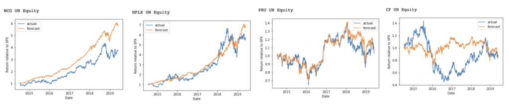
Before diving into Bayesian approaches, I began by calculating factor exposures for every stock in the S\&P500 using a simple linear regression to determine if my price movements could be accurate decomposed into my factors, as suggested in the literature. I observe that this is the case and the mean factor exposures do enable me to decompose returns into specific elements (Figure 1).

Figure 1: Cumulative returns and cumulative returns decomposed into my 8 linear components. We observe that these components are able to fairly accurately now-cast performance. Note that these are not forecasts. The model uses end-of-day feature values to predict end-of-day returns.

However, while this approach seems to work well (and is supported by 50 years of academic literature), all is not as it seems. When I plot the returns of another group of random securities against the factor model decomposition along with the uncertainty of the factor model, I observe a uselessly wide range of outcomes (Figure 2). Over the observed time period, at the upper bound, the price of almost every stock will increase by a factor of 10+, and at the lower bound, fall to zero.

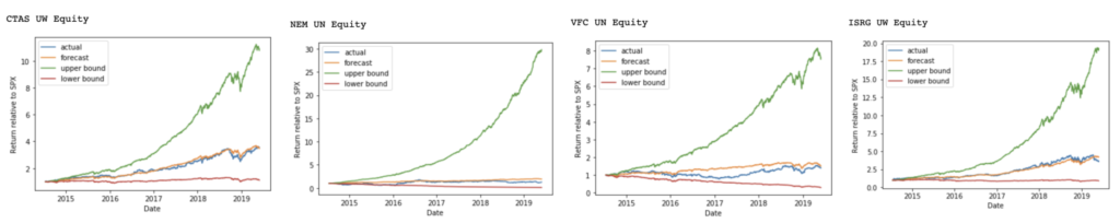
Figure 2: Estimates of return plotted $\pm$ standard error of each factor exposure. Forecasting would be challenging with such wide confidence intervals.

Thus, while the frequentist approach may prove useful for now-casting and analysis, better understanding of uncertainty is required to make forecasts based on the factor model. For this, I turn to Bayesian approaches.

Bayesian Approach

To get a better understanding of the uncertainty of the factor model, I switch to a Bayesian approach. Rather than computing the factor exposures for each security using a linear regression, I assume that each day’s return is drawn from a normal distribution centered on a linear combination of all of the factors.

$r \sim \mathcal{N}(\mu, \sigma)$ where $\mu=\alpha + \beta_{market} + \beta_{size} + \beta_{value} + \beta_{momentum} + \beta_{volatility} + \beta_{yield} + \beta_{active-to-passive} +\beta_{ep}$ , $\pi(\beta) = \mathcal{N}(0,1000)$ , and $\pi(\sigma)=HalfCauchy(10)$ .

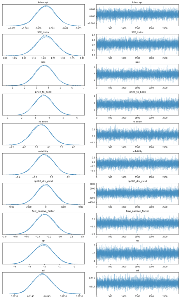
Using these priors and the observed return and factors data, I sampled the posterior using 4, 3,000-link chains with PyMC3 and observed good convergence across that handful of securities that I verified by hand (Figure 3) (Salvatier 2016)

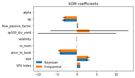
Figure 3: Sample of MCMC chains for Facebook (FB) returns. We see good convergence after 3,000 iterations.

I then compared the Bayesian and frequentist means and standard deviations of the factor exposures for several securities. I observed that they were largely identical. Figure 4 shows the values for ExxonMobil for reference.

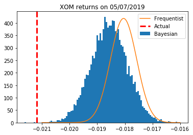
Figure 4: Mean and standard deviation factor exposures for Exxon-Mobil. coefficient. Note that the values are quite similar for every factor.

To investigate further, I compared a distribution of returns sampled from the posterior with the actual values and a frequentist prediction based on the least-squares regression (Figure 5). Not surprisingly, the distributions, like the factor exposures, were qualitatively identical in that no portfolio manager would adjust a decision based on their differences. Notably, for this day, the actual return did not fall within 99th percentile of either distribution! While I show XOM as a representative sample, every other ticker behaved in a similar fashion.

Figure 5: Mean and standard deviation factor exposures for Exxon-Mobil. coefficient. Note that the values are quite similar for every factor.

Conclusions

The original point of this project was to show how an analyst might use Bayesian statistics to improve returns forecasting using Fama-French-inspired factor models. However, I have shown the opposite. The factor exposures generated through Bayesian methods converge to essentially the same values as those calculated using a simple, fast ordinary least squares regression.

While practitioners could use Bayesian linear regressions to calculate factor exposures and use posterior sampling to forecast future returns, those posterior are qualitatively captured through frequentist statistics. Further, computing the mean and standard deviation of every factor exposure for every stock in the S\&P500 for a four-year period requires seconds via least squared regression versus hours for Bayesian sampling techniques. Thus, for this particular application, frequentist statistics are adequate, which explains why they are used widely in the literature and in industry.

In retrospect, these conclusions make total sense. We know that the value of Bayesian inference lies in small sample sizes and strong priors. In finance, we have hundreds of arguably independent samples (daily returns) and weak priors. The Bayesian solution should sensibly converge to the frequentist one. I fleetingly thought about swapping normal priors for something with fatter tails to force the model to consider Black-Swan-style events but realized that with so many examples, the priors are essentially cast aside. In the future, I believe that Bayesian statistics can be applied successfully to rare events like crises and pandemics but not the everyday forecasting of stock returns.

References

Fama, Eugene F., and Kenneth R. French. “Common risk factors in the returns on stocks and bonds.” Journal of (1993).

Fama, Eugene F., and Kenneth R. French. “A five-factor asset pricing model.” Journal of financial economics 116.1 (2015): 1-22.

Qian, Edward E., Ronald H. Hua, and Eric H. Sorensen. Quantitative equity portfolio management: modern techniques and applications. CRC Press, 2007.

Salvatier, John, Thomas V. Wiecki, and Christopher Fonnesbeck. “Probabilistic programming in Python using PyMC3.” PeerJ Computer Science 2 (2016): e55.

Sharpe, William F. “Capital asset prices: A theory of market equilibrium under conditions of risk.” The journal of finance 19.3 (1964): 425-442.