I spend most of my working hours thinking about automatic speech recognition, i.e. teaching machines like Alexa and Siri to transform speech into text. This is a devilishly hard problem that has challenged researchers for almost a century and led to a number of interesting breakthroughs in signal processing and machine learning. While state-of-the-art speech recognition systems rely on sophisticated algorithms and tens of thousands of hours of labeled data, in the not-too-distant past, reasonable performance could be attained with relatively simple classical machine learning algorithms. As part of a class exercise, I applied many of these to the acoustic modeling task and like my results enough to share here.

Introduction to automatic speech recognition

Humans have been trying to teach machines to recognize natural speech since the early days of AI research. In the 1920s, Bell Labs researchers calculated that transmitting telephone conversations across the Atlantic would require ten times the bandwidth available on the existing telegraph cables. A proposed solution was to recognize a speaker’s words and syllables and reconstruct them on the listener’s end without transmitting the temporally and spectrally redundant information associated with natural speech (Atal 2005). These early vocoder efforts have evolved into modern speech recognition technologies that power the now-ubiquitous voice assistants that increasingly penetrate our everyday lives.

The traditional speech recognition task involves predicting a sequence of words from a raw audio signal. This task is typically broken down into feature extraction, where some kind of Fourier transform is used to generate a time series of frequency-based vectors to represent the signal, alignment, where those individual frames are aligned to a specific part of a word, acoustic modeling, where a function created to maps acoustic frames to word fragments, and language modeling, where those word fragments are assembled into complete words and sentences. The ASR research community actively studies all four of these areas, but for the sake of this assignment, I will focus on the acoustic modeling piece.

Using the open-source Kaldi library (Povey 2011), I extracted the features and alignments from the common LibriSpeech benchmark (Panayotov 2016). The features are 80-dimensional vectors representing signal amplitude at 80 different bands of frequencies (log-mel filter banks) (Davis 1980). Each 10 millisecond, 80-dimensional frame, is force aligned with a reference sequence of three letters (chenones) through the Kaldi bootstrapping procedure (Le 2019, Panayotov 2016). This yields a sequence of 80-dimensional vectors and 1-dimensional targets (combinations of three letters). However, because I will be working with a small segment of the LibriSpeech corpus due to computational restraints, I removed all non-speech frames and distilled the thousands of three-letter targets into 26 single-letter ones. While both of these decisions would dramatically impact the quality of a full ASR system (mo’ data, mo’ better and ‘a’ in ‘car’ sounds different than ‘a’ in California), they make exploring the performance of different learners feasible given the resources available.

Unsupervised data exploration

Before beginning work on supervised learning, I wanted to spend some time exploring the data. The LibriSpeech dataset contains nearly a thousand hours of labeled audiobook recordings (Panayotov 2015). Each segment is assigned to a split (train, dev, test), classified by difficulty (clean, other), and a speaker label that includes an ID and gender. State-of-the-art models correctly transcribe more than 90% of the words, but given my constraints on model/data size and task (acoustic model only), I wanted to select the cleanest subset of the data that I could train on my laptop, the 8-hour test-clean tranche (Lüscher 2019).

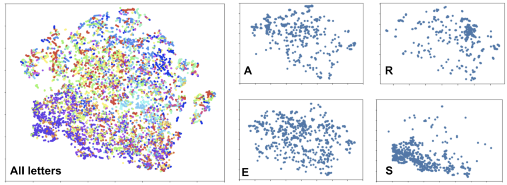
However, while clean by modern ASR standards, the data were quite messy by machine-learning-student standards. The t-SNE plot below provides a small window into how challenging the task of speech recognition really is. Most letters achieve little-to-no-separation from one another.

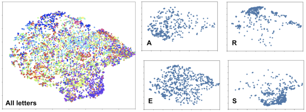
For my learners to accomplish anything, my data needed to get cleaner. Traditional ASR systems rely on phonemes (sounds) rather than graphemes (letters) as targets. I hypothesized that if I replaced my grapheme, ‘e’, with the phonemes associated with that grapheme (e, i, ɛ, ə, etc.), I would see additional separation. However, that replacement process involves training a grapheme-to-phoneme model and realigning the features based on the output of that model, which was beyond the scope of this project. Instead, I segmented the dataset by speaker, hypothesizing that much of the variance could be due to different speaker genders, accents, and idiosyncratic pronunciations.

I sampled 100k frames from each speaker with more than 200 utterances and measured the accuracy of a simple logistic regression model for each subset. Based on the results, I identified Male #220 as the clearest LibriSpeech speaker and reassembled my dataset based on his recordings. This yielded the t-SNE plots below. While some letters are still very challenging to separate, the distribution across many tightens significantly.

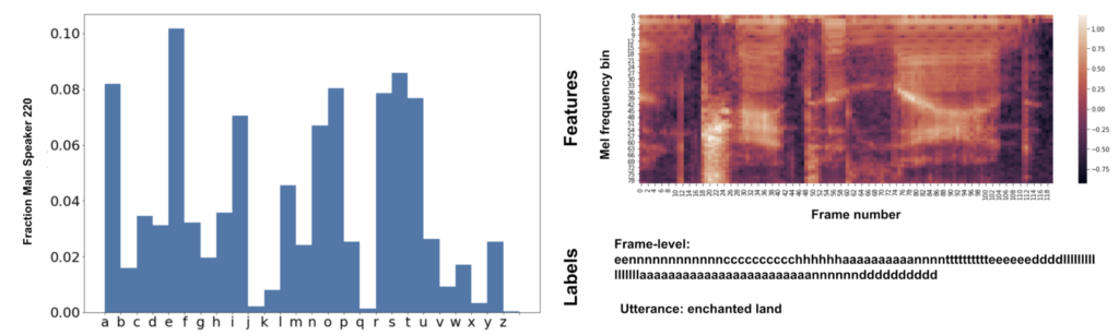
This tranche of Librispeech contains 314,016 frames or around 4 hours of audio. The distribution of labels is unbalanced but qualitatively representative of the English language with ‘e’ representing 10.2% of the labels and ‘z’ 0.04%. However, unlike some unbalanced problems, correctly transcribing an ‘e’ is just as important as correctly transcribing a ‘z’, so there is no need to weight classes by frequency or evaluate performance by more complex metrics. Finally, 90% of the data were assigned to the train split and the balance to the test split. A dev split was omitted because the focus of this assignment is on understanding the machine learning algorithms rather than maximizing performance on a test set via hyperparameter optimization.

Logistic regression

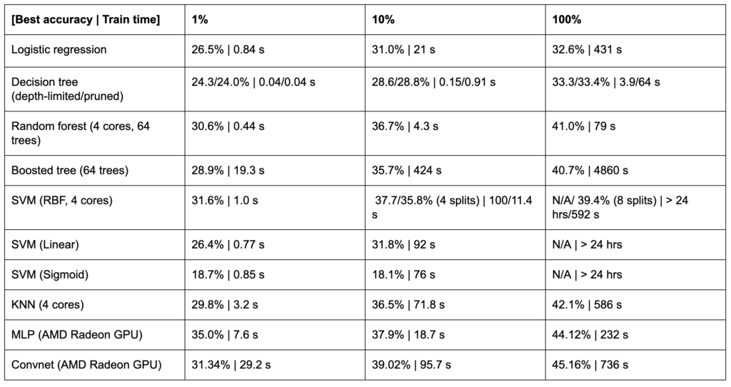
I begin by establishing a baseline with the logistic regression algorithm, which is easily interpretable and can help explain structure in the dataset. When trained on 1%, 10%, and 100% of the train data, this model achieves an accuracy of 26.5%, 31.0%, and 32.6%, respectively. Given that the maximum a posteriori estimation (mode of the posterior), of this distribution is ‘e’, the best random accuracy we could hope for would be 10.2%. These initial logistic regression numbers show that the learner is able to capture significant signals from a small slice of data and gains little from further training.

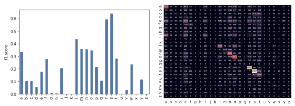
This intuition is confirmed by the two figures above. We see that the logistic regression learner is able to achieve quite reasonable performance on the classes that we observed to be more linearly separable via t-SNE (‘r’, ‘s’, etc.) and poorly on those that were not (‘e’, etc.). When we examine the coefficient weights in Figure 5, we see that the ‘e’ coefficients are all small. The ‘e’ sound is likely too complex for the logistic regression algorithm to model. The ‘r’ sound on the other hand (and many other high-performing classes) is characterized by a single large coefficient over a certain frequency. This explains why the model is able to get 2.5x performance of a random guess from such a small slice of the data. The model is simply learning characteristic frequencies for the easily separable classes.

The confusion matrix tells a similar story. Vowels are frequently confused for one another. An ‘e’ in the dataset is classified as an ‘i’ or an ‘a’ as its true label. Our rare letters like ‘z’, ‘y’, ‘x’, ‘q’, and ‘v’ and more likely to be classified as their most common phonetically similar neighbor, ‘s’, ‘i’, ‘s’, ‘c’, and ‘f’, respectively, than correctly.

Decision tree

The decision tree algorithm may capture some of the non-linearities that our t-SNE plots showed us appear in our data. Using the same 1%, 10%, and 100% splits described previously, I constructed a series of decision trees of various depths using the Scikit-Learn library and split from a subset of random features on Gini impurity (Pedregosa 2011).

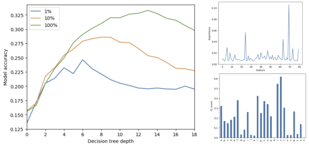
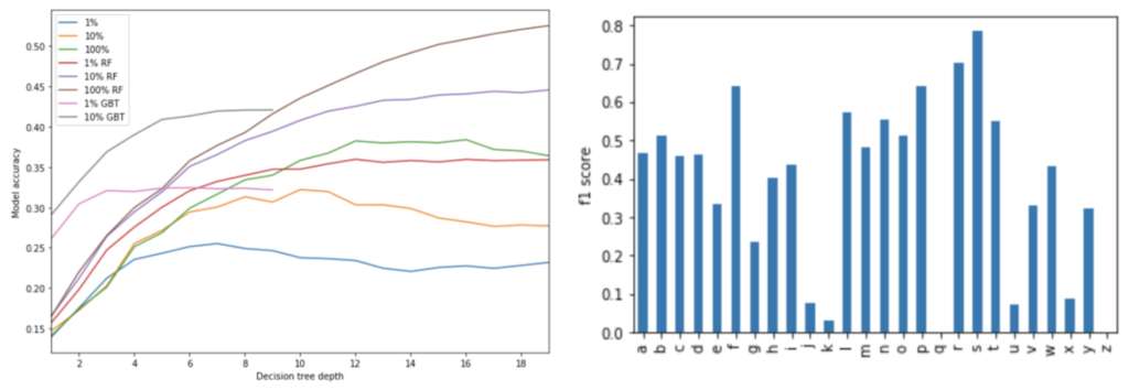
Figure 6 shows that increasing the expressiveness (and thus VC dimension) of the tree improves test set accuracy until a point and that this point can be extended with the inclusion of more data. The best-performing decision tree achieved a 33.2% overall accuracy, which is essentially identical to our logistic regression. However, the distribution of errors was spread more evenly across labels. Performance on the top classes suffered slightly, but our tree was able to correctly label rare letters like ‘j’ and ‘x’, while our logistic regression could only identify the obviously linearly separable classes. We can begin to see this in the feature importance plot that shows that the decision tree heavily weights a number of mel frequencies rather than the one or two that dominated the logistic regression.

While in the previous experiment, we regularized our decision tree by limiting the depth, we can also do the reverse, i.e. grow a full tree and prune nodes that add little to classification accuracy. Here, we use the cost complexity algorithm, which minimizes an equation that contains terms representing the number of leaves and model performance (Breiman 1984).

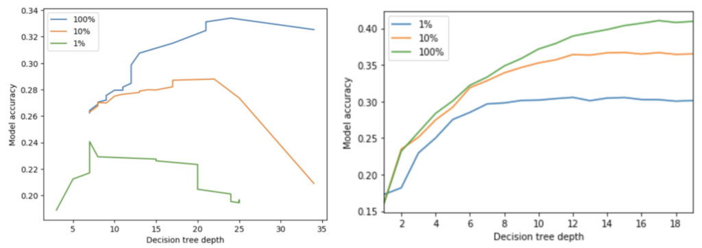
By setting a parameter that scales the weight of the number of leaves and thus increasing or decreasing that term’s relative weight in the cost complexity equation, I either more or less aggressively prune away less important leaves. Interestingly, this post-fit pruning approach yields nearly identical performance (33.3% vs. 33.4% accuracy) to setting the tree depth ahead of time at the expense of greatly increased computational cost (4s vs. 64 s). While peak performance is shifted to the right, i.e. maximum accuracy is achieved with a deeper tree, for this dataset, pruning is not the best strategy to help overcome the fixed horizon problem present in depth-limited trees.

A more effective method to increase the performance of a decision tree is to build a random forest, i.e. an ensemble of many trees trained on different subsets of data. As shown in Figure 7, I repeated the previous experiments using an ensemble of 64 trees and observed an immediate 23% improvement in performance (33.4% vs. 41.0%) with a similar distribution in class-level accuracy. This performance is coupled by a reduced susceptibility to overfitting due to the randomness injected into both training data and features. Even better, because each random decision tree is selected from an independently selectly basket of features at each node and learns from a randomly selected subset of the data, the random forest algorithm is embarrassingly parallel. Using a standard 4-core laptop, a 64 tree forest only requires only slightly more than 16x the wall clock time.

Boosting

In addition to creating a parallel ensemble like a random forest, we can also boost our decision tree. In this case, we train a series of decision trees where each feature/label pair is weighted by the previous model’s performance on the pair. In theory, this lets the model learn from its mistakes and has been shown to outperform the random forest algorithms in many industrial settings (see Kaggle leaderboards). However, because the boosting algorithm is serial rather than parallel and considers performance on each feature independently, it runs very slowly for large, multiclass datasets like this one.

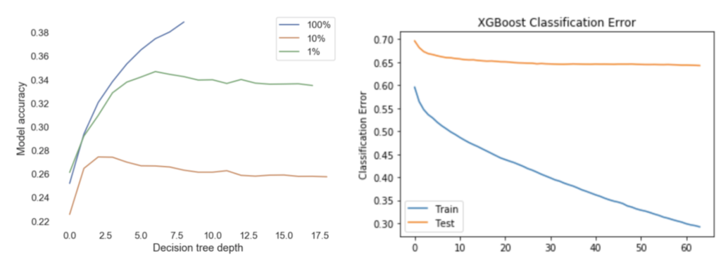
When using XGBoost, one of the faster python libraries for boosting, training a 64-tree ensemble to depth 3 (optimal performance) takes 19.3 s or nearly 100x longer than the equivalent random forest while delivering worse performance (28.9% vs. 30.6%) (Chen 2016). Training a 64-tree ensemble to depth 8 required more than an hour and barely matched the random forest performance. While it is possible to accelerate boosting algorithms by tuning learning rate, subsampling, and training ensembles in parallel, these early results showed that boosted trees are not able to represent this dataset any better than their bagged brethren and require an impractical amount of time to train on this multiclass dataset. Some efforts have been made to improve boosting performance on multiclass problems by replacing classes with class vectors at the leaf (and thus avoiding having to train n-class new trees at each stage), but exploring that algorithm was beyond the scope of this assignment (Ponomareva 2017).

Support vector machine

The SVM algorithm paired with the correct kernel should be able to optimally classify a continuous function. However, this performance comes at a cost. The computational time of the SVM algorithm scales with the cube of the number of samples, O(n3). Fitting 1% of the dataset with the RBF kernel, a popular function for SVM classification which exponentiates Euclidean distance, required 1 second and produced, as expected, the best results with that tranche of data (31.6% accuracy) (Chang 2010). Including 10% required 100 s and also achieved the best accuracy on that set (37.7%). I would fully expect that an SVM paired with the RBF kernel trained on the full dataset would outperform all of the other classical ML algorithms, but the cubic complexity means a single run ought to require more than 24 hrs of wall time. For fun, I left my computer churning on the problem an entire day confirmed that hypothesis.

In an attempt to overcome the cubic computational complexity, I trained several SVMs in parallel and ensembled their results. When split into 4 chunks, the 10% slice trained 10 times faster at the expense of 5% accuracy. Scaling up, I split the entire dataset into 8 chunks and achieved a sub-random-forest 39.4% accuracy in 592 s.

I also experimented with a linear kernel, which should produce nearly identical results to the logistic regression algorithm discussed previously, and the sigmoid kernel, which should replicate the performance of a two-layer MLP and foreshadow the next section. Not surprisingly, the linear kernel numbers were within 3% of the logistic regression. However, the sigmoid function underperformed every other algorithm.

k-nearest neighbors

The KNN classifier should perform similarly to a very deep random forest or SVM. However, instead of partitioning the space with a series of splits ahead of time, the algorithm identifies neighbors based on some distance metric (Euclidean in our case) and predicts a class based on some voting method (each neighbor given uniform weight in our case). This leads to a collection of class islands whose boundaries likely closely resemble the boundaries established by the SVM or random forest algorithm.

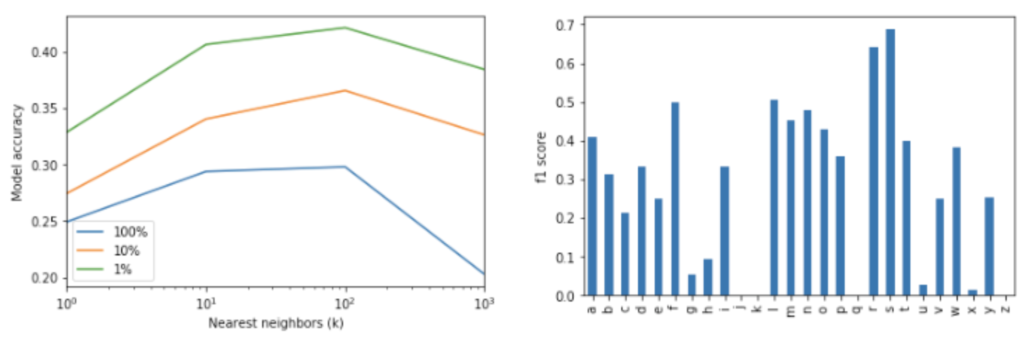
On the speech dataset, KNN achieves the best performance out of all of the traditional ML algorithms. I suspect that this is due to its ability to more easily handle the discontinuities between classes caused by multiple phonemes mapping to the same grapheme. The best decision tree performed 3x better on the best classes (‘s’, ‘r’, etc.) than the middle classes (‘b’,’c’, etc.), but the best KNN reduces that gap to 2x. If we return to the t-SNE plot in the first section, we can see that ‘r’ (and many other letters) exhibits a strong primary cluster with 2-3 secondary ones. Eager learners that partition the space ahead of time may have difficulty with these discontinuities, while the lazy KNN algorithm simply reads off the nearest points. To this point, while the KNN performs very well, the cost of performance is paid at each prediction. Because recognizing a spoken utterance requires analyzing thousands of frames, fast inference is greatly preferred over fast training. The KNN algorithm does the reverse, ao it could never be used for real-world speech recognition tasks.

Unlike the previous algorithms, increasing the data available to the KNN model does not allow us to improve performance by increasing the expressiveness of the model (lowering k). I also attribute this characteristic to the learner style. If the data are distributed relatively uniformly, more data should simply reduce the error bounds because neighboring points are more likely to be closer to the point in question and have little effect on the impact of model expressiveness.

Multilayer perceptron

A two or more layer MLP can theoretically represent any function. Given the complex, non-linear, and discontinuous mapping between acoustic frames and letters, a neural network should outperform the more traditional machine learning algorithms. I confirmed this experimentally. Given the Keras toolkit, fairly vanilla model architecture (128/512/1024/512/128 hidden layers, Adam optimizer, ReLu activation) and little to no tuning, I achieved 44.1% accuracy, 7.5% better than closest practical algorithm (random forest) and 4.8% better than the KNN in a couple minutes on a standard laptop (Chollet 2015). I have no doubt that this performance could be improved significantly with more structured architecture exploration and hyperparameter tuning.

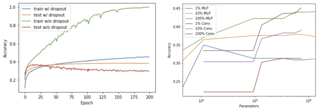
This strong performance trickled down to the smaller datasets as well with the MLP beating every other algorithm by wide margins. Interestingly, the ideal model size varies with the size of the training data. A smaller model with fewer layers actually outperforms a larger model when trained on small subsets of data. This is likely due to a combination of excess model capacity and undertraining, because I fixed each run at 100 epochs.

I also examined the impact of training iteration on test set accuracy. Without the dropout regularization technique, model training must be halted immediately after achieving maximum test-set performance. With 50% dropout on each layer, training can continue nearly indefinitely without decreased test set performance as we observed with the boosting algorithm (Srivastava 2014).

1D-convolutional neural network

While MLPs perform well, they ignore a key piece of information–filter banks are adjacent to one another both in the feature vector and the physical world. In other words, position 56 in the feature is close in frequency space to position 57. Given that we don’t always speak in the same tones, different frequency combinations can actually represent the same letter. Using a convolutional architecture, we can capture relationships between filterbanks and bubble them up to a final classification. By replacing a few MLP layers with 2- or 4-kernel convolutions and 2-unit pooling operations, I was able to improve performance another 2% to 45.16% while simultaneously reducing model size by 50%. As with the MLP, I am confident that these numbers could improve significantly with tuning.

Introduction to the sequence dataset

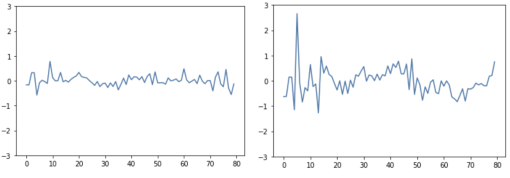
When comparing the performance of our best classifier to the reference labels, something obvious immediately leaps out: the majority of frames are simply the repeat of their predecessor (see Figure 3). By considering each 10 ms frame as an independent event, we are ignoring the clearest structure in this dataset. In fact, when I train a simple bigram language model using the NLTK package on the train set labels, I am able to achieve a 75% accuracy on the test set (Bird 2009). In other words, the preceding label provides far more information than the acoustic frame itself.

In production ASR systems, this history is captured through both providing the acoustic model with an sliding window of context and incorporating word and letter probabilities via a lexicon and language model, but here we will focus entirely on the first approach. For our second dataset, I will study 7-frame windows of acoustic features and attempt to predict the 4th label in the sequence.

Logistic regression

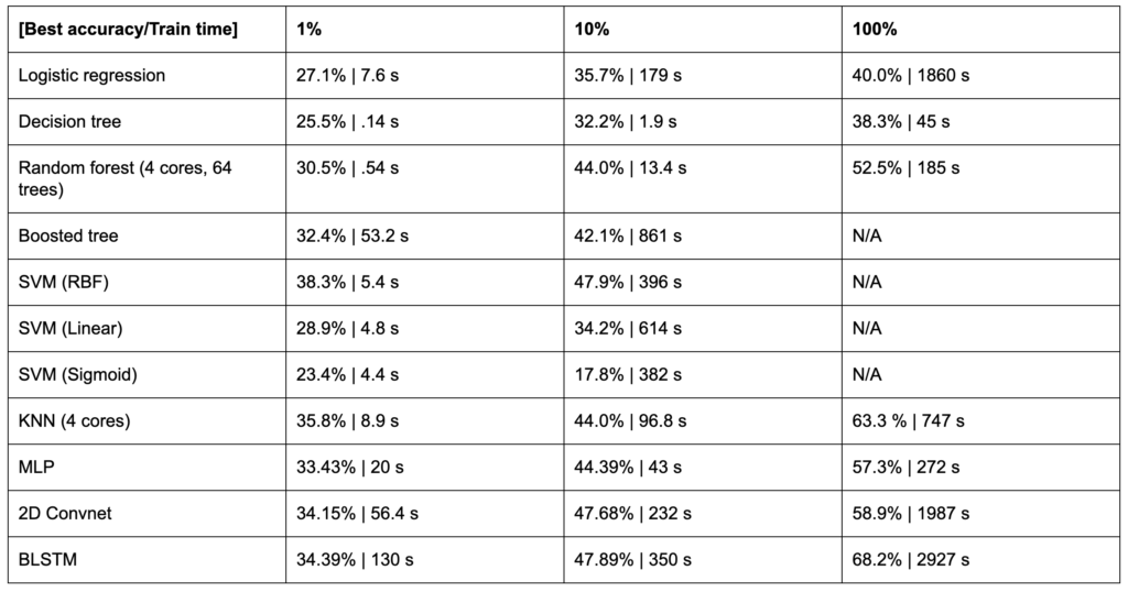
I reran the baseline experiments with the expanded features expecting poor performance. The logistic regression algorithm assumes feature independence, absence of collinearity, and a number of other statistical niceties (Stoltzfus 2011). Given the strongly autoregressive nature of this dataset, I fully expected needing to hand engineer features like sums of differences between frames commonly used in classical speech recognition algorithms (Kumar 2011). However, the logistic regression algorithm overcame its assumptions and improved full-dataset accuracy by 23% (32.6% to 40.0%). More surprising, when I swapped the flattened 7-frame feature for a hand-crafted delta feature pulled straight from the speech recognition literature, performance suffered! While I can’t explain why these correlated features perform so well, I can confirm that the logistic regression model benefits significantly from additional context. Therefore, I will continue to use the raw flattened 7-frame features for the remainder of classical machine learning discussion and discard the idea of engineered delta features.

Decision tree, random forest, and boosted tree

The decision tree algorithm and its boosted and bagged cousins also benefit greatly from the improved context. While the logistic regression improved 23%, the random forest increased that to 28%. Though these algorithms still have no notion of the relationship between frames, i.e. there is not inherent ordering, they still are able to split up the space in a way that takes strong advantage of the sequential nature of the features. Intuitively, this makes sense. A decision tree could gain some certainty from splitting on feature 794 (79th position in middle frame) and augment that certainty by also splitting on 793 and 79*5 given that these frames will likely contain similar acoustic fingerprints.

Again, the random forest outperformed either individual decision trees or gradient boosted trees with only marginally more compute time. Thus far, the random forest is the algorithm to beat in terms of performance, speed, simplicity, and explainability. The best random forest algorithm still struggled with rarer classes like ‘j’, ‘k’, and ‘x’, which is likely due to the discontinuous nature of the dataset.

Support vector machine

The RBF-kernel SVM also benefited greatly (27%) from the sequence of frames improving performance to 47.9% when trained on just 10% of the dataset. Again, I am confident that this algorithm could achieve a classical ML record if it had access to the entire dataset, but the exponential complexity prevented me from training any larger models. As before, linear kernel performance essentially matched the logistic regression numbers above, as expected, and the sigmoidal kernel failed to separate the data much better than a random guess.

k-nearest neighbors

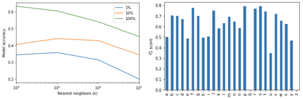
Again, the KNN algorithm outperformed all of the other classical algorithms. Accuracy improved around 20% on the smaller datasets, indicating that the KNN was able to leverage the sequence information about as efficiently as the other algorithms, but rocketed up to 50% for the full-dataset to 63.3% accuracy, the best yet. Interestingly, this is achieved at k=1. Where previously the model began to overfit below k=100, when the dataset becomes large enough (the sequence dataset is effectively 7 times larger than the frame-level one), the space becomes dense enough to achieve good results by reading off a single nearest neighbor. I see this to a lesser effect on the 1% and 10% datasets where maximum performance occurs at k=10 rather than k=100.

MLP, 2D convolutions, and BLSTM

While the algorithms previously discussed all benefited mightily from sequential context, none of them explicitly linked frame 1 to frame 2 to frame 3 and so. Each considered each acoustic feature in each frame as an independent observation. They obviously learned to recognize some of the structure in the dataset, I as the algorithm designer was unable to provide explicit sequencing.

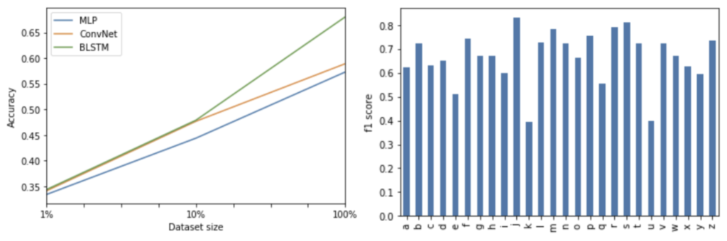
This notion of feature independence changes with the introduction of neural networks. The MLP, as introduced previously, does not explicitly sequence the features, but as before, establishes a reasonable neural baseline of 57.5% on the entire dataset (second place behind k=1 KNN). However, here I introduce two new algorithms, the 2D-convolutional neural net (ConvNet) and the bidirectional long-short term memory recurrent neural net (BLSTM). The 2D ConvNet extends the 1D ConvNet by pooling across both features and time. Thus, the network is able to learn both the spectral relationship between log mels and the temporal relationship between frames (LeCun 1998). The BLSTM uses the hidden state of the previous hidden unit as a feature in the current one to explicitly pass along past information into the future and enforce order onto a sequential dataset (Hochreiter 1997).

These algorithms perform extraordinarily well, achieving first and second place on the speech recognition task. In addition to their strong overall performance, class-level performance is much more uniform. The best KNN not only loses 7% accuracy over the BLSTM but totally fails to correctly label a single ‘q’ or ‘z’. The BLSTM achieved not only 68.2% accuracy but also relatively even class-wise performance without any specific weighting and fast inference. In other words, it has a large enough VC dimension to partition this complex, non-linear, discontinuous space the way that no other models do.

Conclusions

Speech recognition is an extremely challenging machine learning learning task that involves converting variable-length sequences of raw audio to words across a range of acoustic conditions. Here, we explored how algorithms that are best able to capture the sequential nature of adjacent frames, the spectral relationship between different features, and the large discontinuities across the label manifold perform best for this task. However, despite all that work, a simple bigram language model trained on letters alone does far better than our fancy BLSTM acoustic model. In the future, we could significantly improve the performance of our system by considering external data like the structure and vocabulary of the English language.

Frame-level results

Sequence results

References

Atal, Bishnu. Speech and Audio Processing for Coding, Enhancement and Recognition, Chapter 1: From “Harmonic Telegraph” to Cellular Phones. Springer, 2015 pp. 7.

Bird, Steven; Ewan, Klein; Loper, Edwaard; Natural Language

Processing with Python, O’Reilly, 2009.

Chang, Yin-Wen; Hsieh, Cho-Jui; Chang, Kai-Wei; Ringgaard, Michael; Lin, Chih-Jen.Training and Testing Low-degree Polynomial Data Mappings via Linear SVM. Journal of Machine Learning Research, 2010.

Chen, Tianqi; Guestrin, Carlos. XGBoost: A Scalable Tree Boosting System. KDD, 2016.

Chollet, François, et al. Keras. https://keras.io, 2015.

Breiman, Leo; Friedman, Jerome; Olshen, Richard; Stone, Charles. Classification and Regression Trees. Wadsworth, Belmont, CA, 1984.

David, Steven; Mermelstein, Paul. Comparison of Parametric Representations for Monosyllabic Word Recognition in Continuously Spoken Sentences, ICASSP, 1980.

Droppo, Jasha; Seltzer, Michael; Acero, Alex; Chiu, Yu-Hsiang; Towards a Non-Parametric Acoustic Model: An Acoustic Decision Tree for Observation Probability. Interspeech, 2008.

Kumar, Kshitiz; Kim, Chanwoo; Stern, Richard. Delta-spectral cepstral coefficients for robust speech recognition. ICASSP, 2011.

Hochreiter, Sepp; Schmidhuber, Jürgen. Long Short-Term Memory. Neural Computation, 1997.

Le, Duc; Zhang, Xiaohui; Zheng, Weiyi; Fugen, Christian; Zweig, Geoffrey; Seltzer, Michael; From Senones to Chenones: Tied Context-Dependent Graphemes for Hybrid Speech Recognition, ASRU, 2019.

LeCun, Yan; Bottou, Léon; Bengio, Yoshua; Haffner, Patrick. Gradient-based learning applied to document recognition. Proceedings of the IEEE, 1998.

Lüscher Christoph; Beck, Eugen; Irie, Kazuki; Kitza Markus; Michel, Wilfried; Zeyer, Albert; Schlüter, Ralf; Ney, Hermann; RWTH ASR Systems for LibriSpeech: Hybrid vs Attention — w/o Data Augmentation, Interspeech, 2019.

Panayotov, Vassil; Chen, Guoguo; Povey, Daniel; Khudanpur, Sanjeev; LibriSpeech: An ASR Corpus Based on Public-Domain Audiobooks, ICASSP, 2015.

Pedregosa, Fabian et al. Scikit-learn: Machine learning in Python. Journal of Machine Learning Research, 2011.

Ponomareva, Natalia; Colthurst, Thomas; Hendry, Gilbert; Haykal, Salem; Radpour, Soroush; Compact Multi-Class Boosted Trees, IEEE Big Data, 2017.

Povey, Daniel; Ghoshal, Arnab; Boulianne, Gilles; Burget, Lukas; Glembek, Ondrej; Goel, Nagendra; Hannemann, Mirko; Motlicek, Petr; Qian, Yanmin; Schwarz, Petr; Silovsky, Jan; Stemmer, Georg; Vesely, Karel; The Kaldi Speech Recognition Toolkit, ICASSP, 2011.

Srivastava, Nitish; Geoffrey Hinton; Alex Krizhevsky; Ilya Sutskever; Ruslan Salakhutdinov; Dropout: a simple way to prevent neural networks from overfitting, The journal of machine learning research, 2014.

Stoltzfus, Jill. Logistic Regression: A Brief Primer. Academic Emergency Medicine, 2011.