And so it began

I have always been interested finance. Depending on when I were asked, this interest would range from being interested in burning down Wall Street to being interested in starting a hedge fund. However, this interest was largely abstract. Until I moved to California, I had never met anyone who truly worked in finance and I had absolutely no idea about how the industry worked. Part of the reason I joined Orbital Insight last year was to change that.

As any good product manager would, immediately after joining, I began to reach out to friends and friends of friends who worked in various flavors to finance to learn a little bit about their problems at work. I interviewed corn traders who just wished they could get a peek at yield estimates between monthly USDA WASDE reports. I interviewed insurance executives who just wished they knew what kind insane structures their clients were constructing in hurricane-prone regions. I interviewed currency speculators who just wished they knew how large infrastructure projects in the developing world were progressing ahead of government reports. It was all intriguing stuff, so I was taken aback when I interviewed perhaps the most intriguing trader of them all and he only wanted to talk about cryptocurrency.

He was bored with predicting reservoir levels in Pakistan to expose mis-priced OTC pea swaps. Writing computer vision pipelines to analyze road conditions in Brazil to forecast soy exports was mundane. Instead, he was fascinated with decentralized currencies and thought this guy in Silicon Valley might know something about them.

Unfortunately for him, my only exposure to cryptocurrencies came through teasing a kooky friend who had spent the summer proselytizing BTC. However, I was quickly sold. And this wasn’t a sell on the direction or future of cryptocurrencies. I had no particular perspective on whether a sequence of numbers in a shared ledger somehow represented the future of finance and currency. No, this was a sell on profiting from a new, fucked-up market that hadn’t been tamed by Wall Street traders like him yet. We fired a few emails back and forth to share blog posts detailing all of the ridiculous things that were happening at that point (Fall 2017) in the crypto markets and laid plans for our first attempt at riches.

Interexchange arbitrage

In October of 2017, dabblers in cryptocurrency were faced with a curious fact: the price of an individual asset varied across exchanges. Those well-versed in finance will read this sentence in disbelief. There is no sane reason why an asset that costs nothing to transport should be selling for different prices in different markets. However, the crypto exchanges were not sane. Mature markets are full of rational actors arbitraging away nonsense like this, which is why an S&P 500 future in Chicago costs exactly the same as a basket of its underlying stocks in New York, but those rational actors had not yet invaded the crypto markets.

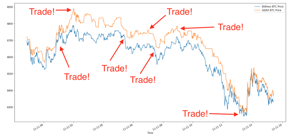
After looking at the figure above for a minute, an obvious trading strategy emerges. The difference between the BTC price on GDAX and the Bitfinex seems to oscillate between $0 and $100 over some random intraday time periods. If we bought BTC with USD on GDAX at the minimum gap and sold at the maximum gap (and did the reverse on Bitfinex), we would make around a hundred bucks a trade and dozens of such trades were available every day! We are leaving out some details regarding execution, BTC long exposure, and interexchange transfers, but a merely clever person with a free AWS instance can work this out. This is in sharp contrast to the established markets where profiting from pure arbitrage requires several PhDs in physics and access to millions of dollars in hardware.

We worked through the exact strategy and set it in code. It backtested beautifully. Using the exact same logic, we fired a few manual orders through the system to make sure we weren’t missing anything. We weren’t. Free money was materializing before our very eyes. Soon, we would throw off the shackles of labor forever!

A week later, we were ready to go. We plumbed our trading logic into an execution unit that posted orders via HTTP requests to various exchange APIs. Wary of holding too large of a long BTC position or too much cash on any of the exchanges, we also included a recycle leg that involved transferring both between exchanges. This was a mistake. Nearly immediately after hitting go, transactions froze.

Early December 2017 was the peak of crypto mania. After a couple profitable trades, our recycle leg activated and fired half our treasury in BTC from Bitfinex to GDAX. As soon as the block was confirmed, we would be ready to go again and keep that arbitrage machine humming. But we waited. And waited. Our trading machine ground to a halt. The BTC network had become so congested that simple BTC transactions were taking days or weeks and only those with mining rigs could push them through. As the days passed, renting a miner to unstick our transaction became a real option, but finally by some good graces the BTC appears in our GDAX account. We had made exactly two trades in nearly a week.

Sloshing dollars and Bitcoins between exchanges and accounts was clearly not going to work. We ran a few experiments by hand to accelerate the recycle loop, but none were satisfying. Then it hit us. Asset transfer was unnecessary. Simply keeping a balance of BTC and USD on two or more exchanges and buying and selling as prices converged and diverged yielded essentially the same result as a traditional pairs trade.

Reinvigorated, we tweaked our code and killed the villainous recycle leg. We finally had it but were too little, too late. By the time we modified our code and backtested the new strategy, the opportunity had evaporated. Those previously juicy $20-$100 price gaps between major exchanges had been reduced to a handful of dollars. A serious arbitrageur could surely pick up some of those Washingtons ahead of the crypto steam roller, but we were out.

Bellman-Ford

Undeterred, we knew that we were only beginning. Just because the most obvious arbitrage opportunity on the planet dried up did not mean that institutional sharks had gobbled up all of the free money that crazed retail investors had left on the table. Earlier in our exploration, we read a post about intra-exchange arbitrage on decentralized exchanges. Essentially, these exchanges don’t have a matching engine, so occasionally a resting bid order will come in below the best ask. One only needs to hit them both at the same time to harvest risk-free profits (interestingly, these strategies still exist if you play with gas prices!). We knew that FX traders still use shortest-path algorithms like Dijkstra’s or Bellman-Ford to identify arbitrage opportunities while trading real currencies, so we hypothesized that the same must exist in the crypto markets.

Unlike the interexchange arbitrage example above, creating an interexchange arbitrage strategy was much more challenging. It is impossible to identify opportunities by eye. Collecting enough data and writing a backtest would take as long as writing the actual system, and much of the risk lies in proper order execution. And we knew that we were strapped for time. We saw the interexchange opportunity collapse in a handful of months. We cobbled together a system using our old HTTP-based order execution module, some devilishly complex data processing steps, and the networkx graph analysis library and unleashed its might on GDAX.

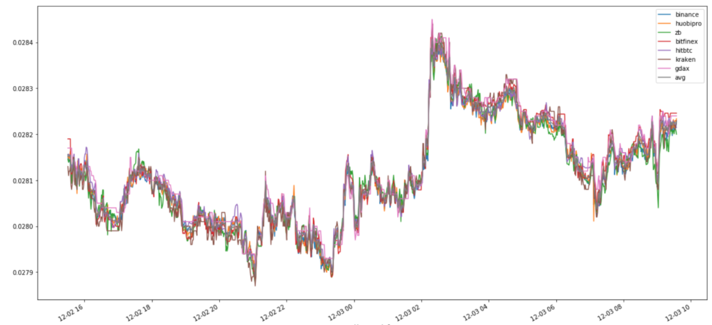
Nothing happened. After a few days of running Bellman-Ford, we didn’t identify a single arbitrage opportunity. At that point (mid-January 2018), only a handful of pairs were available on GDAX, bid/ask spreads had fallen to one cent, and I had a lurking suspicion that Coinbase itself was providing liquidity. While we preferred GDAX for its legitimacy, Bellman-Ford’s shot at fame and fortune lay in the the shadier corners of the crypto world.

A broad spectrum of cryptocurrency exchanges exist. On one hand, there are professional outfits like GDAX and Gemini that are based in the US and have taken serious institutional money to build a serious product. On the other, there are shady decentralized exchanges like EtherDelta that are so bug-ridden that executing a single order can be a challenge in itself. To find opportunities, we needed an exchange with enough crosses to generate mispricings and enough liquidity to keep bid/ask spreads reasonable, but unsophisticated enough that the exchange itself wasn’t running any kind of arbitrage engine itself. In addition, the exchange needed a stable API and ideally would not instill fear every time we deposited currency. With these criteria in mind, we identified Hitbtc, “the most advanced Bitcoin exchange”, as our next target. Bid/ask spreads were small but not too small. 430+ crosses were supported. Liquidity appeared to be real.

We tore out our old execution engine, replaced it with one powered with ccxt, allowing us to abstract away individual exchange peculiarities, and set Bellman-Ford to work. Watching the initial trades like a hawk, we were blown away. $.05 appeared beneath our noses. Then another $0.03. Despite making our requests from a server in the US over HTTP with an 8-second roundtrip, we were profitably arbing a major cryptocurrency exchange. 2 hours later, we had made $10–the hardest $10 I have ever made in my life.

There were several obvious problems with our system, the first being speed. Modern HFT firms construct microwave towers to obtain microsecond advantages when arbing Chicago S&P futures against the NY stocks. Our code used HTTP requests to fetch complete copies 430 order books from across an ocean. This is the equivalent of sending a pigeon from Chicago to NY to report price movements. The fact that we were able to profitably trade 8-second-old opportunities was just loony.

Modern trading firms co-locate their servers with those of the exchanges to reduce the time between receiving price information and executing a trade based on that information. Through some handy profiling experiments, I determined that HTTP request latency was by-far the largest driver of our 8-second roundtrip time. Due to the structure of the Hitbtc API, we had to make an individual HTTP request for each cross. This meant that we made hundreds of requests to assemble our graph. They were made asynchronously, but 430+ requests to a suboptimal server across the Atlantic will always be slow. While a detailed exploration into the benefits of async vs. threading vs. multiprocessing would come later, it was obvious that our first priority should be cutting down on that trip.

We knew that Hitbtc was British, but a little network snooping taught us that their exchange servers were located in German DigitalOcean datacenter. Fortunately, AWS opened a region in Frankfurt, so we could experiment with pseudo-colocalization by simply moving our code there. A couple clicks in the AWS console later, we were trading live with a 1.5-second roundtrip time!

We thought that our problems had been solved. Initial experiments showed that we were running 5x faster and finding arbitrage opportunities every few minutes. As our trust in the system grew, we ran it for steadily longer periods of time with steadily less supervision. Nothing was more satisfying watching free money announce itself in the console as a reward for our mathematical guile. After a few weeks of progress and debugging, we were ready for an unsupervised weekend. Friday night, we started trading and pledged not to look until Sunday.

When Sunday arrived, I thought I had made a mistake. At this point, we had essentially no logging or debugging infrastructure and the fluctuating crypto prices made profitability analysis challenging, but we appeared to have lost around $100 on a few thousand trades. How was this possible? We only traded 0.5%+ profit opportunities including transaction costs. What crazy bug was still lurking in our system?

Thus began a solid month of debugging. This is only of marginal interest for the purposes of this post, but I’ll just say that it involved building a full market simulation system for offline experimentation, robust logging infrastructure for tracking execution of our orders, and quite a few other features that were essentially unrelated to arbitrage. While debugging, we would periodically turn on Bellman-Ford for a few hours at a time. Sometimes we made money, sometimes we lost it. A clear pattern never emerged.

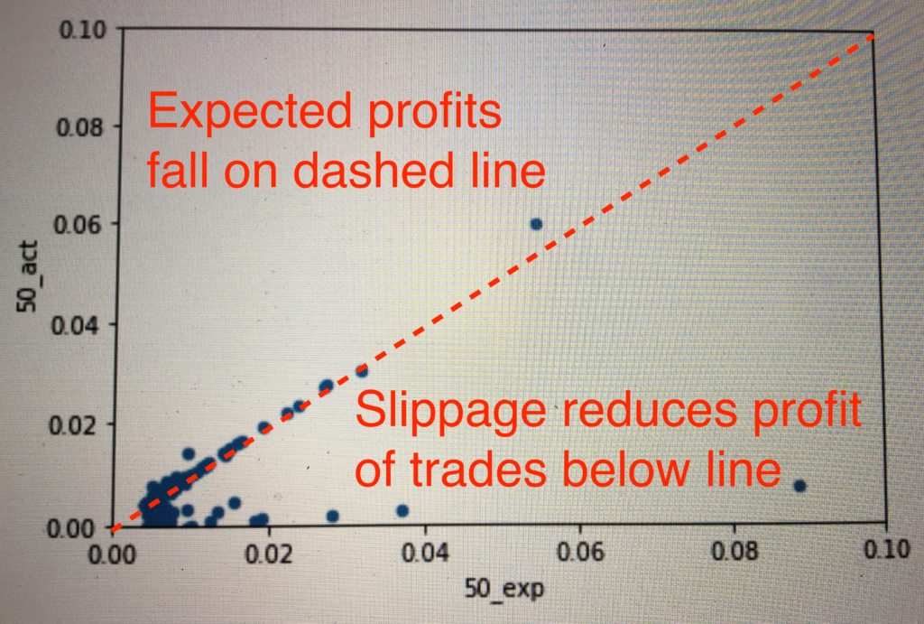
Finally, we solved the mystery. A new type of logging enabled us to compare the expected and actual return of each trade in percentage points. This may sound simple and obvious, but with 430 different crosses, extremely volatile prices and bid/ask spreads, unsynchronized time stamps, and previous evidence that suggested otherwise, it was not.

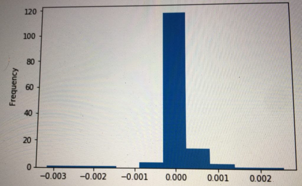
The plot below shows the expected profit (%) per trade versus the actual profit per trade, including transaction costs. If all trades fell on the dotted red line (expected profit = actual profit), we would be making around $500 per day. However, many trades slipped below, reducing our profit potential. In some kind of twisted Pareto distribution, the vast majority of our trades executed as expected (this also contributed to the difficulty in debugging), a handful slipped but remained profitable, and few dozen lost money. Unfortunately, the distribution of trade size was reverse that of trade volume, i.e. a strong inverse correlation existed between trade size and execution quality. In short, while we made money on 99%+ of our trades, the 1% sunk the overall P&L.

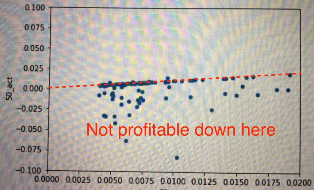
Upon further investigation with our new logging tools, we identified a pattern. The head currencies (BTC, ETH, BCH, etc.) were generally priced very efficiently. Arbitrage opportunities arose when a large order came through a tail currency. If we snapped it up first, we could close the loop and make money. If not, we would get stuck with some weird currency we didn’t want or end up unloading it for an unfavorable price. As before, the game ultimately came down to speed. While in early January we were able to profit with 8 seconds of latency, 1.5 seconds was costing us by March. However, we were fast enough to detect $500 of profit per day on Hitbtc alone. If we were able to speed up our system to the speed of the exchange itself, that prize would be ours for the taking.

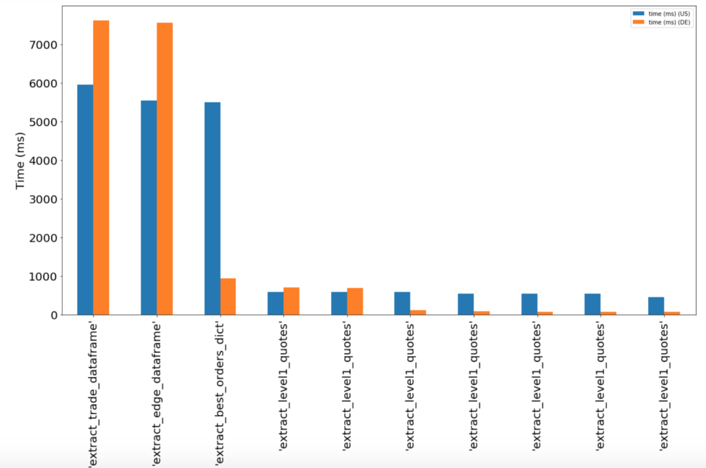
We had a need for speed, but neither of us knew where to start. Books like High Performance Python and Concurrency in Go started appearing on the doorstep. Articles on optimization began dominating my browser history. We knew that our code could be improved in two core areas–I/O and processing. At the time, the I/O modules, including both data collection and order execution, were written in Python using asyncio. Each HTTP request was taking about 500 ms from our German server, but all 430 crosses were taking nearly twice that. In theory, through multiprocessing and multithreading, we should be able to drop the total time to that of the longest individual request. This would give us a solid 500 milliseconds.

On the processing side, we had a few slow steps. We assembled the graph using Pandas, which is slow as molasses and ran graph processing on numpy and networkx. It was dead obvious we needed to change the former. Pandas is nice for analysis, but switching the pipeline to numpy would easily give us a 100x improvement and 200 ms. The latter two were trickier. It would be quite a feat to write our own graph processing functions and along the way, I learned that super-optimized C code is hiding behind numpy’s nice python API and the slow networkx steps very efficiently leverage Python’s fastest data structure.

Many hours later, our optimized code was ready for experimentation. We had dropped the round trip time to an average of 500 ms by running multithreaded requests across multiple machines and excising the slow Pandas operations. But we still weren’t there. At 500 ms, some of our trades were still slipping. We needed to do more.

As a brief aside, there is not much written either online or offline about optimizing HTTP request speed. Several blog posts proclaim the speed benefits of asyncio over threading, but in practice, I observed better average performance using Python’s native multithreading library over asyncio. In addition, writing multithreaded code is much easier than asynchronous code. I wish I kept more careful notes, but I ran experiments comparing multithreading with async across multiple processors and multiple machines. I found that the multiprocessing library almost always slowed things down, but multiple machines (7) using multiple threads and interacting over HTTP (flask) were able to reliably fetch the order books faster than any other combination.

Websockets had been top-of-mind since the beginning. Pulling data from a real-time stream will always be faster than periodic snapshots, but our beloved ccxt library did not yet support websockets, I had literally zero experience in the area, and we would need to write a bunch of complex logic to create the order book itself. I can’t emphasize the challenges of the last point enough. Each Hitbtc HTTP response contains a complete copy of the order book (levels at every price), but each websocket message merely transmits whether market order was filled, a limit order placed, or a limit order canceled. The trader is responsible for maintaining a local copy of the order book and not missing a single message. Missing even a single market order could result in an out-of-date local order book, which could trigger a catastrophic sequence of money losing trades. How? Imagine that the local book missed a message for a cross that rarely traded, meaning quite a bit of time passes between messages. If a theoretical arbitrage opportunity emerged from that missed message, i.e. our local order book identified a arb that was actually not a arb, our highly tuned, 500 ms roundtrip time system, would continue firing unprofitable trades into the exchange at 2 Hz until an updated message came in or a human babysitter pulled the plug. Don’t ask me how I know this 🙂

Challenges aside, the path forward was obvious. For our little operation to have any hope of competing with the other sharks on the exchange, we would need to move at the speed of the exchange. Our first task was to figure out how the heck to create an order book quickly from a stream of messages. This seems easy until you sit down to actually do the task.

Unbeknownst to me, fast order book creation is actually a trade secret that many HFT firms harbor. We discovered this as we began searching for reference implementations and found mostly dead ends and deleted posts. A lead finally emerged thanks to a gentleman named WK Selph. In 2011, he created a WordPress blog on HFT and started writing about various topics including how to build a fast limit order book. However, shortly thereafter someone got word of what he was doing and the blog came down. Fortunately, our friends at the Wayback Machine were able to grab snapshots before the knowledge disappeared forever and some good samaritan in crypto-land even open-sourced a C and Python implementation!

With fast local order book assembly in hand, we got to work on the web socket itself. To this day, I still don’t exactly understand how websockets work, but I want to share our general approach. If a websockets master is reading this and can correct me, please drop me an email. For the sake of curiosity I would love to have a conversation. Anyway, our problem statement was that we wanted to keep up-to-date local order books across 430 crosses using two streams of order placement messages (market and limit) and we couldn’t miss a single message or deal with any queuing.

The naive approach of opening a single websocket failed spectacularly. I don’t exactly recall the message volume, but it was far more than a single websocket on a single machine could handle. Almost immediately, our local order book would begin lagging reality and our arb engine would start firing in bad trades. A second approach was to scale across web sockets. I had switched back to a US server (the websockets stream was faster from the US. I would absolutely love for someone to explain that to me!) and was running an m5.4xl with 8 physical cores and 8 virtual cores. I figured that we could run one websocket per core and eliminate the queuing issue. I allocated 40 crosses to 10 sockets and watched mayhem ensue.

For some reason, whether on the server side or the client side, my websocket feed would not keep up with the market and keeping 10 websockets open on the same machine was not reliable. I tried to balance message volume across sockets and several other tricks, but I never was able to handle bursty periods. Taking inspiration from our previous efforts with HTTP requests, I tried the the same multithreaded, multimachine approach.

Each machine was allocated a block of crosses. Inside each machine, we spun up a handful of threads, on which we opened a single websocket with a handful of crosses balanced by message volume across the whole assembly. Each thread would update the piece of the order book owned by that machine. The whole thing was then wrapped in a flask server that would deliver a piece of the order book when called. When our arbitrage machine fired, it made a request to each machine responsible for collecting data and assembled the complete order book from pieces. This bit of engineering dropped our round trip time to 200 ms. We were finally there.

Determining if we were truly moving at the speed of the exchange was tricky. The we could compare our local order book with the time stamp delivered alongside every complete copy over HTTP, but we didn’t know whether that time stamp was the system time, request time, or delivery time. This really matters when it comes to milliseconds and the Hitbtc team didn’t exactly have a friendly customer service rep that we could call. Instead, we resorted to a great little hack. I recorded our trading console and the Hitbtc UI in slow motion and watched when a price changed. With slow motion video and some patience, I convinced myself we were ready to go.

We popped some champagne and turned on the beast. This was the culmination of months of hard work and learning. We had decreased round trip time by 40x. We would be rich.

Except we weren’t. Our first evening of trading with websockets netted us something like $2.03, which did not even come close to covering the 8-machine AWS bills. Investigating logs, we noticed that all of our trades executed as expected, but there simply wasn’t much arbitrage left to be had. Our competitors were not sitting idle for the months we spent building our system. They too (or Hitbtc for all I know) had supercharged their performance. To provide a sense of closure, I turned off the trading module to measure the remaining arbitrage potential over the weekend–a measly $20/day remained.

Shannon’s Demon

Still stinging from our Bellman-Ford defeat, I picked up Fortune’s Formula by William Poundstone for inspiration. I first became acquainted with this author on Semester at Sea when I picked up Prisoner’s Dilemma: John von Neumann, Game Theory, and the Puzzle of the Bomb, which quickly became my favorite book of all time. I have since read many of his works and casually ordered Fortune’s Formula while exploring Kelly bets for interexchange arb (minor side note: I skipped this in the discussion above, but a critical piece in pairs trading is how much to bet at each inflection point). It is a great read, but one piece in particular struck me.

James Maxwell could be considered the father of statistical mechanics, the physics underlying thermodynamics. As both a physicist and a chemical engineer, both of these subjects are near and dear to my heart. Like Erwin Schrödinger, whose cat appears somewhere in every book peripherally related to quantum mechanics, James Maxwell had an avatar. It was his demon, an operator of a massless door between two chambers filled with gas. The demon could open and close his door between the chambers, letting only the fast gas molecules through and blocking the slow molecules. In theory, this violates the second law of thermodynamics because the demon’s sorting prowess is reducing entropy in a closed system.

Fast forward a century and Claude Shannon reexamined the problem. He argued that the second law was not violated because the decrease in chemical entropy was counteracted by an increase in informational entropy. As the gas molecules are arranged into a more oderly state, fewer bits are required to fully specify this state, thus no physical laws are violated. And this perspective is more than just a thought experiment. We can actually measure the heat released when a large hard drive is erased and the once orderly bits become randomized!

Shannon extended this idea into the markets. What if we had a massless door that let us slosh resources between two uncorrelated assets? This would let us profit from volatility in the markets without taking any bet on the direction of the market. After hedging out long exposure, the only risk would be inflation. Ultimately, Shannon never implemented his demon because volatility in the equities market is too low to result in reasonable volatility pumping profits and transaction costs would swamp out any gains.

Shannon did not live in the time of cryptocurrencies. The volatility in the crypto markets from June 2017 to April 2018 was unlike seen in Shannon’s age. Further the maker/taker model employed by many exchanges, enabled market participants to trade using limit orders free of transaction costs. This structure incentivizes market makers to boost liquidity and encourage other fee-paying (takers) traders to transact. This model is also perfect for implementing Shannon’s demon. Because at its heart Shannon’s demon is a mean reverting strategy (sell on the way up, buy on the way down), execution with limit orders is flawless. The opportunity to implement a theoretical trading strategy inspired by classical statistical mechanics was too much to pass up.

As a reality check, I first ran a simulation. Assuming no transaction costs and near-constant rebalancing, Shannon’s demon would make around 50%/year if the volatility remained constant. Not bad.

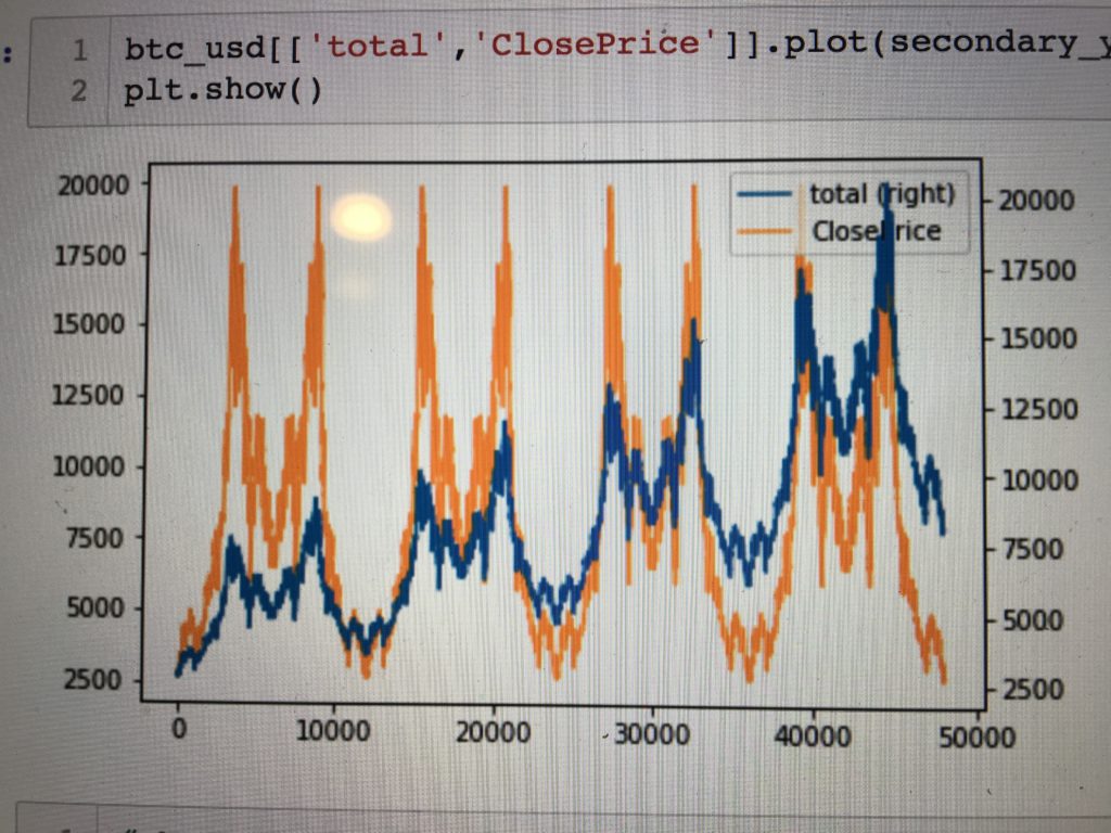
I returned to the trusty execution engine that had already served two other strategies and wrote the 100 lines of code necessary to implement Shannon’s Demon adding a small twist. Rather than just rebalance between cash and BTC, I wanted to rebalance between cash, BTC, ETH, LTC, and BCH, all of the currencies supported on GDAX at that time. My rational was two-fold. First, I thought that I could amplify returns by trading between crypto assets as well as cash. Second, I had been interested in statistical arbitrage since we started this entire experiment. Including a basket of currencies in this strategy was effectively a bet that all four would remain tightly correlated. Historically, the correlations between all of them hovered around .97 and any gap that opened should represent an excellent profit-taking opportunity.

At this point, I had gotten very proficient at deploying new strategies and was up and running in no time. Unlike Bellman-Ford or interexchange arbitrage where many things could go horribly wrong, Shannon’s demon was stable. I was running on GDAX, a trustworthy exchange, and the strategy was so bone-simple that it really couldn’t go wrong. I did neglect to include a short position to match the natural long the portfolio held, which disqualified this strategy from receiving the pure arbitrage label, but I was ok with this. I did want some long exposure to crypto (what if BTC did go to the moon?) and implementing a dynamically adjusting hedge on Bitmex would have introduced a host of other problems.

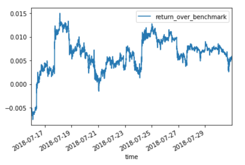
The first month was questionable. Return over benchmark was fluctuating between slightly negative and slightly positive. Including all four currencies in the same basket introduced significant challenges into tracking performance, but I knew that returns would take time. In my backtest, it took Shannon’s Demon a full six months to start to differentiate itself from the buy-and-hold baseline, so I waited patiently.

Shannon’s Demon finally showed his face midway through month two. By simply rebalancing, we had achieved a 1% return over our benchmark! Shannon’s Demon was real. Hell, if we could hedge out our long exposure, it might actually make sense to put more money into this! 6% a year risk-free isn’t bad!

Unfortunately, not 24 hours after taking this snapshot, ETH and BTC became untethered. The stat arb bet that I wanted so badly to make in conjunction with Shannon’s Demon (that BTC/ETH/BCH/LTC would stay highly correlated) blew up. As ETH plummeted, we were selling BTC/LTC/BCH to fund ETH bid orders all the way down. This could be the bet of the century (that ETH would recover) or the end of a strategy. Unfortunately, it was the latter.

I continued running Shannon’s Demon out of morbid curiosity knowing full well that the bet I was monitoring was not on continued volatility but rather ETH’s recovery relative to BTC. However, with generally plummeting crypto prices and my missing long hedge, I decided to shut down after hitting a 30% pre-decided drawdown threshold. While Shannon’s Demon did not live for long, I believe that I may be the only person who has proven his existence in a real market.

Order book pressure

Making the transition from Orbital to Facebook and starting OMSCS at Georgia Tech threw a modest wrench into my trading aspirations. While I continued monitoring Shannon’s Demon, I really didn’t have the bandwidth to research new strategies and the crypto markets were becoming simply less interesting. Even beyond hitting our 30% drawdown, volatility in crypto had fallen to below that of the stock market. Humanity lost interest.

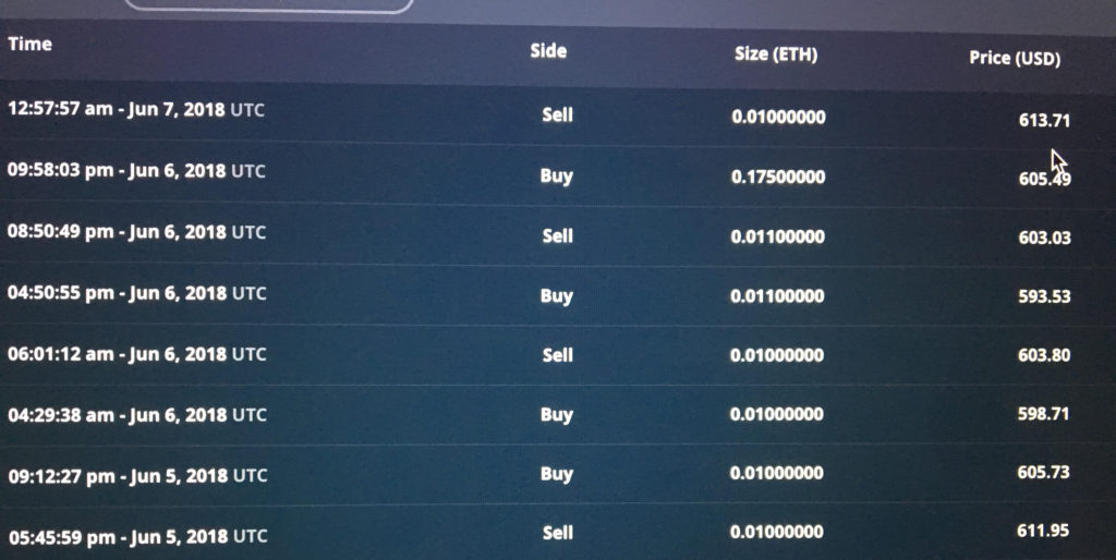
I did have an idea in the back of my mind since I started learning about order books at the start of this whole saga. Information is transmitted to markets in two different ways–market orders and limit orders. The formers sends a strong an immediate message: “Get rid of this asset at any cost. I have a strong perspective that its price will drop.” The former, a more subtle one: “I will let another market participant take this asset off of my hands for the right price.” Forecasting future market movements would be trivial if we could intercept market orders. However, this is both technically infeasible and highly illegal. I believe the feds calls it front-running. Limit orders, however, convey information before they are filled. They rest on the order books until canceled or matched with a market order.

The balance and shape of a limit order book is frequently used in the equities and futures markets to predict future prices. In some sense, it is obvious why. An accumulation of bid orders should indicate an increased interest in an asset, which should correspond to an increased price. This relationship isn’t quite as straightforward as I made it sound, but it serves as a nice mental model.

I have read several interesting papers on order book dynamics and always wanted to replicate some of their results in crypto where limit order books are freely available to recreational traders. An opportunity arose while selecting a final project for Data and Visual Analytics, my Georgia Tech poison of the semester, which is a fantastic class for anyone interested. We had to create a team, collect a novel dataset, and visualize and analyze it in an interesting way. With crypto still on my mind, I pitched Deep Order Book. Using high-frequency order book data we would predict the next price at next tick. While this isn’t technically arbitrage, we did get some nice results, so I wanted to include it here.

We started by simply pulling order book data. Returning to our old trusty friend GDAX, we grabbed snapshots at 3-5 Hz and collected a few days worth of data. After a quick round of processing to convert the raw feed to relative order book snapshots like the beauty below.

We started by trying to predict the next tick’s price movement using a random forest and the raw levels as features. I assumed that this would not work, but I wanted to establish a baseline and understand the relative feature importances of different price levels. I suspected that the best bid and best ask would dominate, but expected deeper orders to signal some kind of intention. I had read that even if deeper orders rarely get executed, they are still useful in determining the direction of the market.

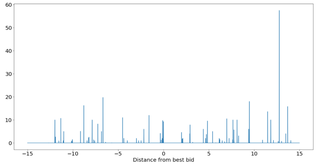
That random forest was able to predict in sample as well as I wanted it to, but overfit horribly to the training set. I suspect that this is due to the highly autocorrelated nature of price data. While I fed the model hundreds of thousands of rows, best bid (my model’s target) did not move for the vast majority of time steps. Even after reducing the tree depth to 3 and batting less than 50% at predicting a positive or negative price movement (at inference time the model got no reward for predicting a constant price), performance on the test set was still dismal. However, the feature importance plot was illuminating. The plot below was generated from an overfitting model of tree depth 5 or so and shows that nearly all of the predictive power of limit orders comes from the first two levels of the book.

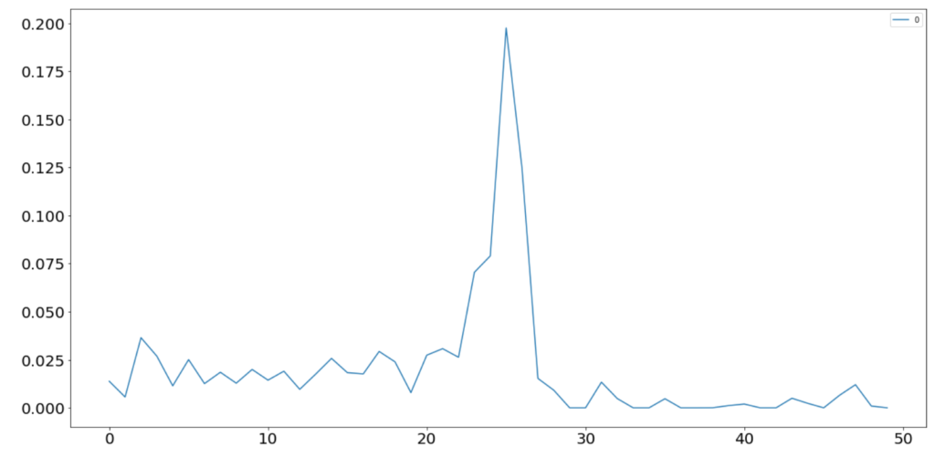
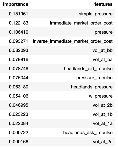
With this in mind and a benchmark set, I began engineering some more interesting features. These were inspired by various HFT papers (and the Headlands Tech blog) and included:

• simple_pressure: best bid volume – best ask volume
• immediate_market_order_cost: best bid volume * best bid price
• pressure: sum of all bids within $0.25 of best – sum of all asks within $0.25 of best
• inverse_immediate_market_order_cost: best ask volume * best ask price
• vol_at_bb: best bid volume
• vol_at_ba: best ask volume
• headland_bid_impulse: best bid volume / trailing average bid volume
• pressure_impulse: headland_pressure – headland_bid_impulse
• w_pressure: pressure vector dot 1/price vector
• headland_ask_impulse: best ask volume / trailing average ask volume

With these features and the same experimental setup, our tree performance on our training set increased to 77% and performance on various out-of-sample test sets stayed consistent in the high 50% to 60% range. This means that with just a simple set of order book features, we can predict the next tick with a better than random chance accuracy.

That said, I’m not sure that this is tradable. Predicting the movement of a rapidly moving market is one thing. Designing a profitable execution strategy that accounts for fees, slippage, other participants, market influence, and the rest is an entirely different challenge. Unfortunately, the semester came to an end before we got there and this idea will have to remain in the ice box until the next opportunity arises.

Thanks for reading this novel of a post and please do reach out if any of this is interesting and you’d like to collaborate on a new project!